objects
| Button | Action |
| Lens | magnify lens |
| Hand | pan zoom |
| data mode | inspect single data points |
| mask data | select data points to mask |
| X | Autoscale X |
| Y | Autoscale Y |
| Z | Autoscale Z |
| + | zoom in |
| - | zoom out |
| Left | Shift all graphs to the left |
| Right | Shift all graphs to the right |
| Up | Shift all graphs up |
| Down | Shift all graphs to the down |
| X+ | Increases magnification in X |
| X- | Decreases magnification in X |
| Y+ | Increases magnification in Y |
| Y- | Decreases magnification in Y |
| Z+ | Increases magnification in Z |
| Z- | Decreases magnification in Z |
| Name | Description | Parameter | Applies to |
| Data set operations | アクティブロットに少なくとも二つのグラフr場合、ダイアログでこのデータセットを操作できます。データセットの加算、減算、掛け算、割り算ができます。 | 二つのデータセット | |
| Average | この関数を用いて、グラフ中のn点の平均がとれます。ポイントの数は1/nに減ります。 | 平均するポイント数 | everything |
| Compress | この関数は、大きなデータセットを少ないポイント数に圧縮できます。合計か平均かにかかわらず、ある数のポイントに関して選択できます。 | 合計、あるいは平均するポイント数 | everything |
| Smooth | この関数は平均に似ていますが、全てのデータポイントに対して機能します。つまり、元のデータの数と同じデータ数をもつ滑らかなグラフが得られます。 | ポイント数 | SPREADSHEET, X-Y, X-Y-DY, X-Y-DX-DY, X-Y-DY-DY, X-Y-Z |
| Prune | この機能はn番目のポイントを使用することで、ポイントデータ数を減少させます。 結果として起こる数は1/nに減少させられます。 | 連続したポイントの数 | SPREADSHEET, X-Y, X-Y-DY, X-Y-DX-DY, X-Y-DY-DY |
| Periodical Functions | この関数は、関数の一つの区間でデータセットを減少させます。合計か平均にかかわらず選択できます。 | 合計/平均; 区間内のポイント数 | SPREADSHEET, X-Y, X-Y-DY, X-Y-DX-DY, X-Y-DY-DY |
| Seasonal | この関数は、ある区間と次の区間の差(あるいは合計)を計算します。区間は、その中のポイント数で指定されます。 | 合計/差; 区間内のポイント数 | SPREADSHEET, X-Y, X-Y-DY, X-Y-DX-DY, X-Y-DY-DY |
| Peak find | この関数は、データセット内のピーク(負のピークも含む)を検出します。 閾値と精度のパラメーターでピーク検出感度を決定できます。 | 正/負のピーク ; 閾値 (Y-Range); 精度 (X-range) |
X-Y, X-Y-DY, X-Y-DX-DY, X-Y-DY-DY |
| Histogram | この関数で、グラフのヒストグラムを作れます。これは、y-軸の範囲をn個に分け、全てのデータポイントをそれらのいずれかに割り当てることを意味します。 | 使われるY-range; binsの数 | SPREADSHEET, X-Y, X-Y-DY, X-Y-DX-DY, X-Y-DY-DY, MATRIX |
| Interpolation | 補間法は与えられたセットのデータポイントを通して滑らかなカーブを見つけようとします。 それをするのに異なったタイプの補間法を使用できます: linear, polynomial, cspline, akima。 すべてのアクティブ領域内のデータポイントが補間に使用されます。 |
補間のtype; 補間関数の範囲/ポイントの数 | SPREADSHEET, X-Y, X-Y-DY, X-Y-DX-DY, X-Y-DY-DY |
| Differences | このダイアログはグラフの一次導関数の近似を作成します。 | None | SPREADSHEET, X-Y, X-Y-DY, X-Y-DX-DY, X-Y-DY-DY |
| Integration | "Show Info" チェックボックスで、積分グラフを加えるかどうか選択できます。この関数は、グラフの数値積分に使われます。 "Add Graph"チェックボックスが選択されていると、、累積合計が別窓に表示されます。 | ベースライン/積分範囲; 合計あるいは面積 (absolute values) |
SPREADSHEET, X-Y, X-Y-DY, X-Y-DX-DY, X-Y-DY-DY |
| Regression | 回帰関数は10次までの多項式でグラフのフィットが行えます。 | 重み/モデル; ポイントの数/回帰関数の範囲 | X-Y,X-Y-DY,X-Y-DX-DY |
| Fourier Tansform | この関数で、グラフの フーリエ変換が計算できます。LabPlotはfftwかgslライブラリを使用できます。 前方変換か後方変換を選択できます。 |
X-values:index/frequency/period; Y-values:magnitude/phase/real part/imaginary part | X-Y, X-Y-DY, X-Y-DX-DY, X-Y-DY-DY |
Convolution/Deconvolution |
この関数で、一つのグラフの他のグラフへのコンボリューションを計算できます。 LabPlot はgslの FFTを使用します。また、セットのデコンボリューションも可能です。 | X-values:index/same as signal | X-Y, X-Y-DY, X-Y-DY-DY + X-Y, X-Y-DY, X-Y-DY-DY |
| Nonlinear Fit | この関数でグラフを非線形フィットできます。12の異なったモデル、あるいは最大9パラメータのユーザー定義関数が選択できます。指数関数モデルは特に初期値に敏感であることに注意してください。フィットの結果のパラ メータはボトムフィールドに示され、さらなるフィットのため初期 値と自動的に取り替 えられます。 結果はラベルとしてプロットに追加されます。 |
fit function;initial values;baseline/region for fitting; range/number of points for fit function | X-Y, X-Y-DY, X-Y-DX-DY, X-Y-DY-DY |
| Image Manipulation | この関数で、行列やアクティブプロットのイメージデータ(例えばSurfaceプロット)を操作できます。LabPlotは、およそ50の異なった方法でイメージを変換するためにImageMagickのAPIを使用します。 | size (height/width) of resulting image | MATRIX,IMAGE |
| Function | Description |
| acos(x) | Arc cosine |
| acosh(x) | Arc hyperbolic cosine |
| asin(x) | Arcsine |
| asinh(x) | Arc hyperbolic sine |
| atan(x) | Arctangent |
| atan2(y,x) | arc tangent function of two variables |
| atanh(x) | Arc hyperbolic tangent |
| beta(a,b) | Beta |
| cbrt(x) | Cube root |
| ceil(x) | Truncate upward to integer |
| chbevl(x, coef, N) | Evaluate Chebyshev series |
| chdtrc(df,x) | Complemented Chi square |
| chdtr(df,x) | Chi square distribution |
| chdtri(df,y) | Inverse Chi square |
| cos(x) | Cosine |
| cosh(x) | Hyperbolic cosine |
| cosm1(x) | cos(x)-1 |
| dawsn(x) | Dawson’s integral |
| drand() | Random value between 0..1 |
| ellie(phi,m) | Incomplete elliptic integral (E) |
| ellik(phi,m) | Incomplete elliptic integral (E) |
| ellpe(x) | Complete elliptic integral (E) |
| ellpk(x) | Complete elliptic integral (K) |
| exp(x) | Exponential, base e |
| expm1(x) | exp(x)-1 |
| expn(n,x) | Exponential integral |
| fabs(x) | Absolute value |
| fac(i) | Factorial |
| fdtrc(ia,ib,x) | Complemented F |
| fdtr(ia,ib,x) | F distribution |
| fdtri(ia,ib,y) | Inverse F distribution |
| gdtr(a,b,x) | Gamma distribution |
| gdtrc(a,b,x) | Complemented gamma |
| hyp2f1(a,b,c,x) | Gauss hypergeometric function |
| hyperg(a,b,x) | Confluent hypergeometric 1F1 |
| i0(x) | Modified Bessel, order 0 |
| i0e(x) | Exponentially scaled i0 |
| i1(x) | Modified Bessel, order 1 |
| 1e(x) | i Exponentially scaled i1 |
| igamc(a,x) | Complemented gamma integral |
| igam(a,x) | Incomplete gamma integral |
| igami(a,y0) | Inverse gamma integral |
| ncbet(aa,bb,xx) | i Incomplete beta integral |
| incbi(aa,bb,yy0) | Inverse beta integral |
| Function | Description |
| iv(v,x) | Modified Bessel, nonint. order |
| j0(x) | Bessel, order 0 |
| j1(x) | Bessel, order 1 |
| jn(n,x) | Bessel, order n |
| jv(n,x) | Bessel, noninteger order |
| k0(x) | Mod. Bessel, 3rd kind, order 0 |
| k0e(x) | Exponentially scaled k0 |
| k1(x) | Mod. Bessel, 3rd kind, order 1 |
| k1e(x) | Exponentially scaled k1 |
| kn(nn,x) | Mod. Bessel, 3rd kind, order n |
| lbeta(a,b) | Natural log of |beta| |
| ldexp(x,exp) | multiply floating-point number by integral power of 2 |
| log(x) | Logarithm, base e |
| log10(x) | Logarithm, base 10 |
| logb(x) | radix-independant exponent |
| log1p(x) | log(1+x) |
| ndtr(x) | Normal distribution |
| ndtri(x) | Inverse normal distribution |
| pdtrc(k,m) | Complemented Poisson |
| pdtr(k,m) | Poisson distribution |
| pdtri(k,y) | Inverse Poisson distribution |
| pow(x,y) | power function |
| psi(x) | Psi (digamma) function |
| rand() | Random value between 0..RAND_MAX |
| random() | Random value between 0..RAND_MAX |
| rgamma(x) | Reciprocal Gamma |
| rint(x) | round to nearest integer |
| sin(x) | Sine |
| sinh(x) | Hyperbolic sine |
| spence(x) | Dilogarithm |
| sqrt(x) | Square root |
| stdtr(k,t) | Student’s t distribution |
| stdtri(k,p) | Inverse student’s t distribution |
| struve(v,x) | Struve function |
| tan(x) | Tangent |
| tanh(x) | Hyperbolic tangent |
| true_gamma(x) | true gamma |
| y0(x) | Bessel, second kind, order 0 |
| y1(x) | Bessel, second kind, order 1 |
| yn(n,x) | Bessel, second kind, order n |
| yv(v,x) | Bessel, noninteger order |
| zeta(x,y) | Riemann Zeta function |
| zetac(x) | Two argument zeta function |
| Function | Description |
| gsl_log1p(x) | log(1+x) |
| gsl_expm1(x) | exp(x)-1 |
| gsl_hypot(x,y) | sqrt{x^2 + y^2} |
| gsl_acosh(x) | arccosh(x) |
| gsl_asinh(x) | arcsinh(x) |
| gsl_atanh(x) | arctanh(x) |
| airy_Ai(x) | Airy function Ai(x) |
| airy_Bi(x) | Airy function Bi(x) |
| airy_Ais(x) | scaled version of the Airy function S_A(x) Ai(x) |
| airy_Bis(x) | scaled version of the Airy function S_B(x) Bi(x) |
| airy_Aid(x) | Airy function derivative Ai’(x) |
| airy_Bid(x) | Airy function derivative Bi’(x) |
| airy_Aids(x) | derivative of the scaled Airy function S_A(x) Ai(x) |
| airy_Bids(x) | airy_Bids(x) derivative of the scaled Airy function S_B(x) Bi(x) |
| airy_Bids(x) | airy_Bids(x) derivative of the scaled Airy function S_B(x) Bi(x) |
| airy_Bids(x) | derivative of the scaled Airy function S_B(x) Bi(x) |
| airy_0_Ai(s) | s-th zero of the Airy function Ai(x) |
| airy_0_Bi(s) | s-th zero of the Airy function Bi(x) |
| airy_0_Aid(s) | s-th zero of the Airy function derivative Ai’(x) |
| airy_0_Bid(s) | s-th zero of the Airy function derivative Bi’(x) |
| bessel_JJ0(x) | regular cylindrical Bessel function of zeroth order, J_0(x) |
| bessel_JJ1(x) | regular cylindrical Bessel function of first order, J_1(x) |
| bessel_Jn(n,x) | regular cylindrical Bessel function of order n, J_n(x) |
| bessel_YY0(x) | irregular cylindrical Bessel function of zeroth order, Y_0(x) |
| bessel_YY1(x) | irregular cylindrical Bessel function of first order, Y_1(x) |
| bessel_Yn(n,x) | irregular cylindrical Bessel function of order n, Y_n(x) |
| bessel_I0(x) | regular modified cylindrical Bessel function of zeroth order, I_0(x) |
| bessel_I1(x) | regular modified cylindrical Bessel function of first order, I_1(x) |
| bessel_In(n,x) | regular modified cylindrical Bessel function of order n, I_n(x) |
| bessel_II0s(x) | scaled regular modified cylindrical Bessel function of zeroth order, |
| exp (-|x|) I_0(x) bessel_II1s(x) | scaled regular modified cylindrical Bessel function of first order, |
| exp(-|x|) I_1(x) bessel_Ins(n,x) | scaled regular modified cylindrical Bessel function of order n, |
| exp(-|x|) I_n(x) bessel_K0(x) | irregular modified cylindrical Bessel function of zeroth order, K_0(x) |
| bessel_K1(x) | irregular modified cylindrical Bessel function of first order, K_1(x) |
| bessel_Kn(n,x) | irregular modified cylindrical Bessel function of order n, K_n(x) |
| bessel_KK0s(x) | scaled irregular modified cylindrical Bessel function of zeroth order, |
| exp (x) K_0(x) bessel_KK1s(x) | scaled irregular modified cylindrical Bessel function of first order, |
| exp(x) K_1(x) bessel_Kns(n,x) | scaled irregular modified cylindrical Bessel function of order n, |
| exp(x) K_n(x) | bessel_j0(x) regular spherical Bessel function of zeroth order, j_0(x) |
| bessel_j1(x) | regular spherical Bessel function of first order, j_1(x) |
| bessel_j2(x) | regular spherical Bessel function of second order, j_2(x) |
| bessel_jl(l,x) | regular spherical Bessel function of order l, j_l(x) |
| bessel_y0(x) | irregular spherical Bessel function of zeroth order, y_0(x) |
| bessel_y1(x) | irregular spherical Bessel function of first order, y_1(x) |
| bessel_y2(x) | irregular spherical Bessel function of second order, y_2(x) |
| bessel_yl(l,x) | irregular spherical Bessel function of order l, y_l(x) |
| bessel_i0s(x) | scaled regular modified spherical Bessel function of zeroth order, |
| exp(-|x|) i_0(x) bessel_i1s(x) | scaled regular modified spherical Bessel function of first order, |
| exp(-|x|) i_1(x) bessel_i2s(x) | scaled regular modified spherical Bessel function of second order, |
| exp(-|x|) i_2(x) bessel_ils(l,x) | scaled regular modified spherical Bessel function of order l, exp(-|x|) |
| i_l(x) bessel_k0s(x) | scaled irregular modified spherical Bessel function of zeroth order, |
| exp(x) k_0(x) bessel_k1s(x) | scaled irregular modified spherical Bessel function of first order, |
| exp(x) k_1(x) bessel_k2s(x) | scaled irregular modified spherical Bessel function of second order, |
| exp(x) k_2(x) bessel_kls(l,x) | scaled irregular modified spherical Bessel function of order l, exp(x) |
| k_l(x) bessel_Jnu(nu,x) | regular cylindrical Bessel function of fractional order nu, J_\nu(x) |
| bessel_Ynu(nu,x) | irregular cylindrical Bessel function of fractional order nu, Y_\nu(x) |
| bessel_Inu(nu,x) | regular modified Bessel function of fractional order nu, I_\nu(x) |
| bessel_Inus(nu,x) | scaled regular modified Bessel function of fractional order nu, |
| exp(-|x|) I_\nu(x) bessel_Knu(nu,x) | irregular modified Bessel function of fractional order nu, K_\nu(x) |
| bessel_lnKnu(nu,x) | logarithm of the irregular modified Bessel function of fractional order |
| nu,ln(K_\nu(x)) bessel_Knus(nu,x) | scaled irregular modified Bessel function of fractional order nu, |
| exp(|x|) K_\nu(x) bessel_0_J0(s) | s-th positive zero of the Bessel function J_0(x) |
| bessel_0_J1(s) | s-th positive zero of the Bessel function J_1(x) |
| bessel_0_Jnu(nu,s) | s-th positive zero of the Bessel function J_nu(x) |
| clausen(x) | Clausen integral Cl_2(x) |
| hydrogenicR_1(Z,R) | lowest-order normalized hydrogenic bound state radial wavefunction |
| R_1 := 2Z \sqrt{Z} \exp(-Z r) | hydrogenicR(n,l,Z,R) n-th normalized hydrogenic bound state radial wavefunction |
| dawson(x) | Dawson’s integral |
| debye_1(x) | first-order Debye function D_1(x) = (1/x) \int_0^x dt (t/(e^t - 1)) |
| debye_2(x) | second-order Debye function D_2(x) = (2/x^2) \int_0^x dt (t^2/(e^t -1)) |
| debye_3(x) | third-order Debye function D_3(x) = (3/x^3) \int_0^x dt (t^3/(e^t - 1)) |
| debye_4(x) | fourth-order Debye function D_4(x) = (4/x^4) \int_0^x dt (t^4/(e^t -1)) |
| dilog(x) | dilogarithm |
| ellint_Kc(k) | complete elliptic integral K(k) |
| ellint_Ec(k) | complete elliptic integral E(k) |
| ellint_F(phi,k) | incomplete elliptic integral F(phi,k) |
| ellint_E(phi,k) | incomplete elliptic integral E(phi,k) |
| ellint_P(phi,k,n) | incomplete elliptic integral P(phi,k,n) |
| ellint_D(phi,k,n) | incomplete elliptic integral D(phi,k,n) |
| ellint_RC(x,y) | incomplete elliptic integral RC(x,y) |
| ellint_RD(x,y,z) | incomplete elliptic integral RD(x,y,z) |
| ellint_RF(x,y,z) | incomplete elliptic integral RF(x,y,z) |
| ellint_RJ(x,y,z) | incomplete elliptic integral RJ(x,y,z,p) |
| gsl_erf(x) | error function erf(x) = (2/\sqrt(\pi)) \int_0^x dt \exp(-t^2) |
| gsl_erfc(x) | complementary error function erfc(x) = 1 - erf(x) = (2/\sqrt(\pi)) \int_x^\infty \exp(-t^2) |
| log_erfc(x) | logarithm of the complementary error function \log(\erfc(x)) |
| erf_Z(x) | Gaussian probability function Z(x) = (1/(2\pi)) \exp(-x^2/2) |
| erf_Q(x) | upper tail of the Gaussian probability function Q(x) = (1/(2\pi)) \int_x^\infty dt \exp(-t^2/2) |
| gsl_exp(x) | exponential function |
| exprel(x) | (exp(x)-1)/x using an algorithm that is accurate for small x |
| exprel_2(x) | 2(exp(x)-1-x)/x^2 using an algorithm that is accurate for small x |
| exprel_n(n,x) | n-relative exponential, which is the n-th generalization of the functions ‘gsl_sf_exprel’ |
| exp_int_E1(x) | exponential integral E_1(x), E_1(x) := Re \int_1^\infty dt \exp(-xt)/t |
| exp_int_E2(x) | second-order exponential integral E_2(x), E_2(x) := \Re \int_1^\infty dt \exp(-xt)/t^2 |
| exp_int_Ei(x) | exponential integral E_i(x), Ei(x) := PV(\int_{-x}^\infty dt \exp(-t)/t) |
| shi(x) | Shi(x) = \int_0^x dt sinh(t)/t |
| chi(x) | integral Chi(x) := Re[ gamma_E + log(x) + \int_0^x dt (cosh[t]-1)/t] |
| expint_3(x) | exponential integral Ei_3(x) = \int_0^x dt exp(-t^3) for x >= 0 |
| si(x) | Sine integral Si(x) = \int_0^x dt sin(t)/t |
| ci(x) | Cosine integral Ci(x) = -\int_x^\infty dt cos(t)/t for x > 0 |
| atanint(x) | Arctangent integral AtanInt(x) = \int_0^x dt arctan(t)/t |
| fermi_dirac_m1(x) | complete Fermi-Dirac integral with an index of -1, F_{-1}(x) = e^x / (1 + e^x) |
| fermi_dirac_0(x) | complete Fermi-Dirac integral with an index of 0, F_0(x) = \ln(1 + e^x) |
| fermi_dirac_1(x) |
complete Fermi-Dirac integral with an index of 1, F_1(x) = \int_0^\infty dt (t /(\exp(t-x)+1)) |
| fermi_dirac_2(x) |
complete Fermi-Dirac integral with an index of 2, F_2(x) = (1/2) \int_0^\infty dt (t^2 /(\exp(t-x)+1)) |
| fermi_dirac_int(j,x) |
complete Fermi-Dirac integral with an index of j, F_j(x) = (1/Gamma(j+1)) \int_0^\infty dt (t^j /(exp(t-x)+1)) |
| fermi_dirac_mhalf(x) | complete Fermi-Dirac integral F_{-1/2}(x) |
| fermi_dirac_half(x) | complete Fermi-Dirac integral F_{1/2}(x) |
| fermi_dirac_3half(x) | complete Fermi-Dirac integral F_{3/2}(x) |
| fermi_dirac_inc_0(x,b) |
incomplete Fermi-Dirac integral with an index of zero, F_0(x,b) = \ln(1 + e^{b-x}) - (b-x) |
| gamma(x) | Gamma function |
| lngamma(x) | logarithm of the Gamma function |
| gammastar(x) | regulated Gamma Function \Gamma^*(x) for x > 0 |
| gammainv(x) |
reciprocal of the gamma function, 1/Gamma(x) using the real Lanczos method. |
| taylorcoeff(n,x) | Taylor coefficient x^n / n! for x >= 0 |
| fact(n) | factorial n! |
| doublefact(n) | double factorial n!! = n(n-2)(n-4)... |
| lnfact(n) | logarithm of the factorial of n, log(n!) |
| lndoublefact(n) | logarithm of the double factorial log(n!!) |
| choose(n,m) | combinatorial factor ‘n choose m’ = n!/(m!(n-m)!) |
| lnchoose(n,m) | logarithm of ‘n choose m’ |
| poch(a,x) | Pochhammer symbol (a)_x := \Gamma(a + x)/\Gamma(x) |
| lnpoch(a,x) | logarithm of the Pochhammer symbol (a)_x := \Gamma(a + x)/\Gamma(x) |
| pochrel(a,x) |
relative Pochhammer symbol ((a,x) - 1)/x where (a,x) = (a)_x := \Gamma(a + x)/\Gamma(a) |
| gamma_inc_Q(a,x) |
normalized incomplete Gamma Function P(a,x) = 1/Gamma(a) \int_x\infty dt t^{a-1} exp(-t) for a > 0, x >= 0 |
| gamma_inc_P(a,x) |
complementary normalized incomplete Gamma Function P(a,x) = 1/Gamma(a) \int_0^x dt t^{a-1} exp(-t) for a > 0, x >= 0 |
| gsl_beta(a,b) |
Beta Function, B(a,b) = Gamma(a) Gamma(b)/Gamma(a+b) for a > 0, b > 0 |
| lnbeta(a,b) | logarithm of the Beta Function, log(B(a,b)) for a > 0, b > 0 |
| betainc(a,b,x) | normalize incomplete Beta function B_x(a,b)/B(a,b) for a > 0, b > 0 |
| gegenpoly_1(lambda,x) | Gegenbauer polynomial C^{lambda}_1(x) |
| gegenpoly_2(lambda,x) | Gegenbauer polynomial C^{lambda}_2(x) |
| gegenpoly_3(lambda,x) | Gegenbauer polynomial C^{lambda}_3(x) |
| gegenpoly_n(n,lambda,x) | Gegenbauer polynomial C^{lambda}_n(x) |
| hyperg_0F1(c,x) | hypergeometric function 0F1(c,x) |
| hyperg_1F1i(m,n,x) |
confluent hypergeometric function 1F1(m,n,x) = M(m,n,x) for integer parameters m, n |
| hyperg_1F1(a,b,x) |
confluent hypergeometric function 1F1(m,n,x) = M(m,n,x) for general parameters a,b |
| hyperg_Ui(m,n,x) |
confluent hypergeometric function U(m,n,x) for integer parameters m,n |
| hyperg_U(a,b,x) | confluent hypergeometric function U(a,b,x) |
| hyperg_2F1(a,b,c,x) | Gauss hypergeometric function 2F1(a,b,c,x) |
| hyperg_2F1c(ar,ai,c,x) |
Gauss hypergeometric function 2F1(a_R + i a_I, a_R - i a_I, c, x) with complex parameters |
| hyperg_2F1r(ar,ai,c,x) |
renormalized Gauss hypergeometric function 2F1(a,b,c,x) / Gamma(c) |
| hyperg_2F1cr(ar,ai,c,x) |
renormalized Gauss hypergeometric function 2F1(a_R + i a_I, a_R - i a_I, c, x) / Gamma(c) |
| hyperg_2F0(a,b,x) | hypergeometric function 2F0(a,b,x) |
| laguerre_1(a,x) | generalized Laguerre polynomials L^a_1(x) |
| laguerre_2(a,x) | generalized Laguerre polynomials L^a_2(x) |
| laguerre_3(a,x) | generalized Laguerre polynomials L^a_3(x) |
| lambert_W0(x) | principal branch of the Lambert W function, W_0(x) |
| lambert_Wm1(x) | secondary real-valued branch of the Lambert W function, W_{-1}(x) |
| legendre_P1(x) | Legendre polynomials P_1(x) |
| legendre_P2(x) | Legendre polynomials P_2(x) |
| legendre_P3(x) | Legendre polynomials P_3(x) |
| legendre_Pl(l,x) | Legendre polynomials P_l(x) |
| legendre_Q0(x) | Legendre polynomials Q_0(x) |
| legendre_Q1(x) | Legendre polynomials Q_1(x) |
| legendre_Ql(l,x) | Legendre polynomials Q_l(x) |
| legendre_Plm(l,m,x) | associated Legendre polynomial P_l^m(x) |
| legendre_sphPlm(l,m,x) |
normalized associated Legendre polynomial $\sqrt{(2l+1)/(4\pi)} \sqrt{(l-m)!/(l+m)!} P_l^m(x)$ suitable for use in spherical harmonics |
| conicalP_half(lambda,x) |
irregular Spherical Conical Function P^{1/2}_{-1/2 + i \lambda}(x) for x > -1 |
| conicalP_mhalf(lambda,x) |
regular Spherical Conical Function P^{-1/2}_{-1/2 + i \lambda}(x) for x > -1 |
| conicalP_0(lambda,x) | conical function P^0_{-1/2 + i \lambda}(x) for x > -1 |
| conicalP_1(lambda,x) | conical function P^1_{-1/2 + i \lambda}(x) for x > -1 |
| conicalP_sphreg(l,lambda,x) |
Regular Spherical Conical Function P^{-1/2-l}_{-1/2 + i \lambda}(x) for x > -1, l >= -1 |
| conicalP_cylreg(l,lambda,x) |
Regular Cylindrical Conical Function P^{-m}_{-1/2 + i \lambda}(x) for x > -1, m >= -1 |
| legendre_H3d_0(lambda,eta) |
zeroth radial eigenfunction of the Laplacian on the 3-dimensional hyperbolic space, L^{H3d}_0(lambda,eta) := sin(lambda eta)/(lambda sinh(eta)) for eta >= 0 |
| legendre_H3d_1(lambda,eta) |
zeroth radial eigenfunction of the Laplacian on the 3-dimensional hyperbolic space, L^{H3d}_1(lambda,eta) := 1/sqrt{lambda^2 + 1} sin(lambda eta)/(lambda sinh(eta)) (coth(eta) - lambda cot(lambda eta)) for eta >= 0 |
| legendre_H3d(l,lambda,eta) |
L’th radial eigenfunction of the Laplacian on the 3-dimensional hyperbolic space eta >= 0, l >= 0 |
| gsl_log(x) | logarithm of X |
| loga(x) | logarithm of the magnitude of X, log(|x|) |
| logp(x) | log(1 + x) for x > -1 using an algorithm that is accurate for small x |
| logm(x) | log(1 + x) - x for x > -1 using an algorithm that is accurate for small x |
| gsl_pow(x,n) | power x^n for integer n |
| psii(n) | digamma function psi(n) for positive integer n |
| psi(x) | digamma function psi(n) for general x |
| psiy(y) | real part of the digamma function on the line 1+i y, Re[psi(1 + i y)] |
| ps1i(n) | Trigamma function psi’(n) for positive integer n |
| ps_n(m,x) | polygamma function psi^{(m)}(x) for m >= 0, x > 0 |
| synchrotron_1(x) | first synchrotron function x \int_x^\infty dt K_{5/3}(t) for x >= 0 |
| synchrotron_2(x) | second synchrotron function x K_{2/3}(x) for x >= 0 |
| transport_2(x) | transport function J(2,x) |
| transport_3(x) | transport function J(3,x) |
| transport_4(x) | transport function J(4,x) |
| transport_5(x) | transport function J(5,x) |
| hypot(x,y) | hypotenuse function \sqrt{x^2 + y^2} |
| sinc(x) | sinc(x) = sin(pi x) / (pi x) |
| lnsinh(x) | log(sinh(x)) for x > 0 |
| lncosh(x) | log(cosh(x)) |
| zetai(n) | Riemann zeta function zeta(n) for integer N |
| gsl_zeta(s) | Riemann zeta function zeta(s) for arbitrary s |
| hzeta(s,q) | Hurwitz zeta function zeta(s,q) for s > 1, q > 0 |
| etai(n) | eta function eta(n) for integer n |
| eta(s) | eta function eta(s) for arbitrary s |
| Function | Description |
| gaussian(x,sigma) | probability density p(x) at X for a Gaussian distribution with standard deviation SIGMA |
| ugaussian(x) |
unit Gaussian distribution. They are equivalent to the functions above with a standard deviation of one, SIGMA = 1 |
| gaussian_tail(x,a,sigma) |
probability density p(x) at X for a Gaussian tail distribution with standard deviation SIGMA and lower limit A |
| ugaussian_tail(x,a) |
tail of a unit Gaussian distribution. They are equivalent to the functions above with a standard deviation of one, SIGMA = 1 |
| bivariate_gaussian(x,y,sigma_x,sigma_y,rho) |
probability density p(x,y) at (X,Y) for a bivariate gaussian distribution with standard deviations SIGMA_X, SIGMA_Y and correlation coefficient RHO |
| exponential(x,mu) |
probability density p(x) at X for an exponential distribution with mean MU |
| laplace(x,a) |
probability density p(x) at X for a Laplace distribution with mean A |
| exppow(x,a,b) |
probability density p(x) at X for an exponential power distribution with scale parameter A and exponent B |
| cauchy(x,a) |
probability density p(x) at X for a Cauchy distribution with scale parameter A |
| rayleigh(x,sigma) |
probability density p(x) at X for a Rayleigh distribution with scale parameter SIGMA |
| rayleigh_tail(x,a,sigma) |
probability density p(x) at X for a Rayleigh tail distribution with scale parameter SIGMA and lower limit A |
| landau(x) |
probability density p(x) at X for the Landau distribution |
| gamma_pdf(x,a,b) |
probability density p(x) at X for a gamma distribution with parameters A and B |
| flat(x,a,b) |
probability density p(x) at X for a uniform distribution from A to B |
| lognormal(x,zeta,sigma) |
probability density p(x) at X for a lognormal distribution with parameters ZETA and SIGMA |
| chisq(x,nu) |
probability density p(x) at X for a chi-squared distribution with NU degrees of freedom |
| fdist(x,nu1,nu2) |
probability density p(x) at X for an F-distribution with NU1 and NU2 degrees of freedom |
| tdist(x,nu) |
probability density p(x) at X for a t-distribution with NU degrees of freedom |
| beta_pdf(x,a,b) |
probability density p(x) at X for a beta distribution with parameters A and B |
| logistic(x,a) |
probability density p(x) at X for a logistic distribution with scale parameter A |
| pareto(x,a,b) |
probability density p(x) at X for a Pareto distribution with exponent A and scale B |
| weibull(x,a,b) |
probability density p(x) at X for a Weibull distribution with scale A and exponent B |
| gumbel1(x,a,b) |
probability density p(x) at X for a Type-1 Gumbel distribution with parameters A and B |
| gumbel2(x,a,b) |
probability density p(x) at X for a Type-2 Gumbel distribution with parameters A and B |
| poisson(k,mu) |
probability p(k) of obtaining K from a Poisson distribution with mean mu |
| bernoulli(k,p) |
probability p(k) of obtaining K from a Bernoulli distribution with probability parameter P |
| binomial(k,p,n) |
probability p(k) of obtaining K from a binomial distribution with parameters P and N |
| negative_binomial(k,p,n) |
probability p(k) of obtaining K from a negative binomial distribution with parameters P and N |
| pascal(k,p,n) |
probability p(k) of obtaining K from a Pascal distribution with parameters P and N |
| geometric(k,p) |
probability p(k) of obtaining K from a geometric distribution with probability parameter P |
| hypergeometric(k,n1,n2,t) |
probability p(k) of obtaining K from a hypergeometric distribution with parameters N1, N2, N3 |
| logarithmic(k,p) |
probability p(k) of obtaining K from a logarithmic
distribution with probability parameter P constants |
| PI1 | 1/pi |
| PI2 | 2/pi |
| PISQRT2 | 2/sqrt(pi) |
| E | e |
| LN2 | log_e 2 |
| LN10 | log_e 10 |
| LOG2E | log_2 e |
| LOG10E | log_10 e |
| PI | pi |
| PI_2 | pi/2 |
| PI_4 | pi/4 |
| SQRT2 | sqrt(2) |
| SQRT1_2 | 1/sqrt(2) |
| constants | description |
| c | The speed of light in vacuum |
| mu0 | The permeability of free space |
| e0 | The permittivity of free space |
| Na | Avogadro’s number |
| F | The molar charge of 1 Faraday |
| k | The Boltzmann constant |
| R0 | The molar gas constant |
| V0 | The standard gas volume |
| Gauss | The magnetic field of 1 Gauss |
| mu | The length of 1 micron |
| ha | The area of 1 hectare |
| mph | The speed of 1 mile per hour |
| kmh | The speed of 1 kilometer per hour |
| au | The length of 1 astronomical unit (mean earth-sun distance) |
| G | The gravitational constant |
| ly | The distance of 1 light-year |
| pc | The distance of 1 parsec |
| g | The standard gravitational acceleration on Earth |
| ms | The mass of the Sun |
| e | The charge of the electron |
| eV | The energy of 1 electron volt |
| amu | The unified atomic mass |
| me | The mass of the electron |
| mmu | The mass of the muon |
| mp | The mass of the proton |
| mn | The mass of the neutron |
| alpha | The electromagnetic fine structure constant |
| Ry | The Rydberg constant |
| a0 | The Bohr radius |
| A | The length of 1 angstrom |
| barn | The area of 1 barn |
| muB | The Bohr Magneton |
| muN | The Nuclear Magneton |
| mue | The magnetic moment of the electron |
| mup | The magnetic moment of the proton |
| min | The number of seconds in 1 minute |
| h | The number of seconds in 1 hour |
| d | The number of seconds in 1 day |
| week | The number of seconds in 1 week |
| in | The length of 1 inch |
| ft | The length of 1 foot |
| yard | The length of 1 yard |
| mile | The length of 1 mile |
| mil | The length of 1 mil (1/1000th of an inch) |
| nmile | The length of 1 nautical mile |
| fathom | The length of 1 fathom |
| knot | The speed of 1 knot |
| pt | The length of 1 printer’s point (1/72 inch) |
| texpt | The length of 1 TeX point (1/72.27 inch) |
| acre | The area of 1 acre |
| ltr | The volume of 1 liter |
| us_gallon | The volume of 1 US gallon |
| can_gallon | The volume of 1 Canadian gallon |
| uk_gallon | The volume of 1 UK gallon |
| quart | The volume of 1 quart |
| pint | The volume of 1 pint |
| pound | The mass of 1 pound |
| ounce | The mass of 1 ounce |
| ton | The mass of 1 ton |
| mton | The mass of 1 metric ton (1000 kg) |
| uk_ton | The mass of 1 UK ton |
| troy_ounce | The mass of 1 troy ounce |
| carat | The mass of 1 carat |
| gram_force | The force of 1 gram weight |
| pound_force | The force of 1 pound weight |
| kilepound_force | The force of 1 kilopound weight |
| poundal | The force of 1 poundal |
| cal | The energy of 1 calorie |
| btu | The energy of 1 British Thermal Unit |
| therm | The energy of 1 Therm |
| hp | The power of 1 horsepower |
| bar | The pressure of 1 bar |
| atm | The pressure of 1 standard atmosphere |
| torr | The pressure of 1 torr |
| mhg | The pressure of 1 meter of mercury |
| inhg | The pressure of 1 inch of mercury |
| inh2o | The pressure of 1 inch of water |
| psi | The pressure of 1 pound per square inch |
| poise | The dynamic viscosity of 1 poise |
| stokes | The kinematic viscosity of 1 stokes |
| stilb | The luminance of 1 stilb |
| lumen | The luminous flux of 1 lumen |
| lux | The illuminance of 1 lux |
| phot | The illuminance of 1 phot |
| ftcandle | The illuminance of 1 footcandle |
| lambert | The luminance of 1 lambert |
| ftlambert | The luminance of 1 footlambert |
| curie | The activity of 1 curie |
| roentgen | The exposure of 1 roentgen |
| rad | The absorbed dose of 1 rad |
| Screenshot | Name | Description |
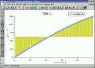
|
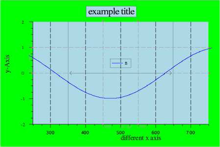
axes label | this example shows how to use different axes label. The shown function is filled to the baseline. |
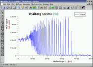
|
rydberg spectra | this example shows a Rydberg spectra measured by photoexcitation of metastable helium in a magneto optical trap. |
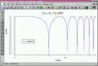
|
log axis scale | this example uses logarithmic axis scales with custom tic label |
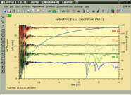
| [IMAGE] | audio data | this example shows data read from an audio file |
| [IMAGE] | marker | this example shows a usage of marker |
|
TeX label | this example uses a TeX label |
|
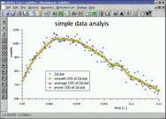
analysis | this example shows the difference between the three analysis functions prune, average and smooth. Here you can see different stylesand symbols for showing data. |
|
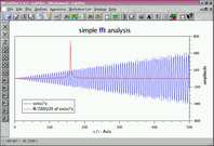
simple fft | this example shows how a simple fourier transform might look like. |
|
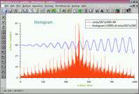
histogram | this example shows a sample histogram of a periodic function. |
|
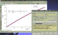
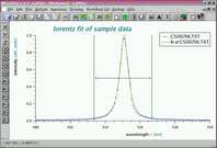
nonlinear fitting | this example shows a nonlinear lorentzian fit of a sample data set in a specified region. |
|
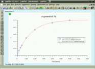
exponential fit | this example shows how an exponential fit of sample data should look like. |
| [IMAGE] | log fit | this example shows an exponential fit inside a logarithmic plot. |
| [IMAGE] | surface | this example shows a simple surface plot with density and contour plot of a used defined function. The color palette is chosen to nicelyshow the function values. |
| [IMAGE] | surface style | this example shows the same data set as surface plot in different styles. |
|
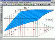
3d | this example shows a simple 3 dimensional plot created from a function. |
|
drawing objects |
this example shows how to use drawing objects in LabPlot. |
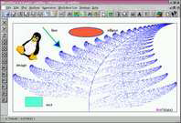
| [IMAGE] | images | this example shows a surface plot created from an image file (utm.xpm). |
|
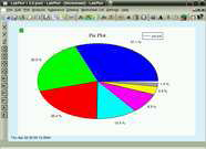
pie plot | this example shows a simple pie plot created from two dimensional data |
| [IMAGE] | bar plot | this example shows the usage of the bar style for x and y ranges. |
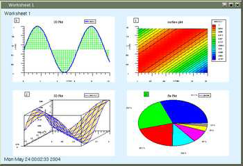
| [IMAGE] | multiple plots | this example shows the usage of multiple plots per worksheet. Here you can s see four different types of plot arranged 2x2 with gap=0.05. |
| [IMAGE] | qwt 3d plot | this example shows the usage of a qwt 3 dimensional plot. This example uses a customized colormap and the "flooriso" style to make the contour lines on the floor. |
| [IMAGE] | another surface plot | this is another example for a surface plot. This example shows how logarithmic axis scales can be used her too. |
| [IMAGE] | polar plot | this example shows a simple polar plot created from functions |
| [IMAGE] | ternary plot | this example shows a ternary plot created with some data |
|
sfi (only on download site) | this example introduces overlayed plots by showing a selective field ionization spectra overlayed with the field ramp. |