1.    Introduction

    A lot of micrometeorological observations using fast response sensors have been carried out to understand the energy and water balances and CO₂ flux on different places. Though different sensors were used, comparisons of these sensors have been rarely seen. During May 14 to 25, 2000, turbulent measurement with 14 different models of sensors, most of which were used in the observations of GAME (GAWEX Asian Monsoon Experiment) projects, was carried out at Terrestrial Environment Research Center (TERC), Universityof Tsukubaby the Flux Enthusiast Party (authors). Our interests are the energy imbalance problem, flux footprint (or source area), methods to evaluateturbulent fluxand comparison of the different turbulent measuring sensors(Toda et al.,2000). The object of this report is focused on comparison of the sensors.

---

2.    Measurement

    Site  The measurement was made at TERCfield.The surface was covered by grass (mainly Solidago altissima,Andropogon virginicusand Equisetum arvence). And thefetch toward the prevailingwind direction(east) was about 100m.
  Sensors  Table 1 lists the installed sensors to compare. Because of bad weather conditions (lightning and heavy rain), only the data obtained by 6 sensors is available. Every open path sensor measures spatial mean properties of the air between probes. The sonic anemothermometers calculates wind speed and air temperature by measuring the speed of sound, and gas analyzers calculate the gas densities by measuring the absorption of infrared radiation. The spans of all the sensors’ probes are 0.12m to 0.2m except closed path sensor. Shorter span sensors enable to measure smaller eddies, but errors are larger. Closed path system pumps the object air into the sampling cells of the sensor through tube, and calculates the gas concentrations by measuring the difference in absorption of infraredradiation passing trough the sample and reference cells. The sensors were installed atheights of 2.5 to 3.3m, and the horizontally distance of eachset was around 0.3m. A sampling frequency set at 10Hz.

Table 1 Available installed sensors.Italics are the abbreviations used in figures.

Set no. (Logger)	Model	Sensor [Object]	Installation height	Span
1(a)	Flux-PAM type*	3D sonic anemothermometer [Temperature]	3.33m	0.15m
2(b)	DA-600-1T**	1D sonic anemothermometer [Temperature]	2.55m	0.20m
3(b)	DA-600-3T**	3D sonic anemothermometer [Temperature]	2.52m	0.20m
1(a)	OP2***	Open path CO2/H2O gas analyzer   [H2O, CO2]	3.30m	0.20m
2(a)	LI-7500****	Open path CO2/H2O gas analyzer   [H2O, CO2]	2.80m	0.12m
1(a)	LI-6262****	Closed path CO2/H2O gas analyzer   [H2O, CO2]	2.85m	(tube)

[Makes] ^*: GILL, ^**: KAIJO, ^***: Data Design Group, ^****: LI-COR

---

3.    Comparison
    It is difficult to compare raw data of the sensors, because each set of sensors is apart horizontally. Thus standard deviations (\sigma) in every 10 minutes were used to make comparisons. The concentrations are converted into the densities.
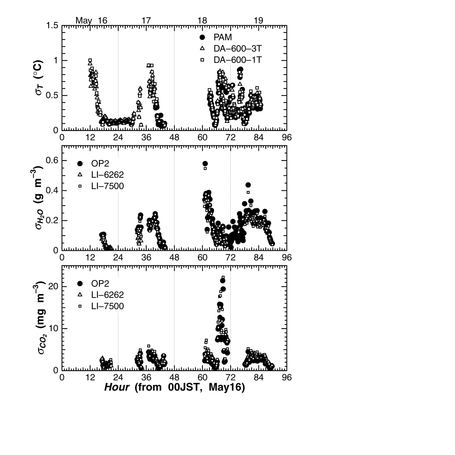
      Fig.1 shows time series on \sigma of the available data. They agree with each other. The weather of the former two days isfiner than the latter, so everys varied more regularly in theformer days.
      Fig.2 shows the relationships between \sigma of the sensors. This figure also shows good agreement of the sensors. Theclosed path LI-6262 sensor is a little smaller in both H ₂O andCO₂ because of the measuring method. Slightly curving relationship between the \sigma of H₂O_OP2 and H ₂O_LI-7500   is seen in this figure, maybe because only theOP2’s H₂O sensor has 2nd order calibration coefficient (othershave only linear). LI-7500’s calibration coefficients are questionable, therefore \sigma of CO_{2 LI-7500}  seems quite larger. However the root mean square error (RMSE) of two open path sensors seems smallenough. These results mean thatthe sensors in this reportare good to usetogether, although not only absolute quantities but also \sigma calibration should be made before flux observations using different turbulent measuring sensors.

---

Acknowledgments  The authors would like to thank KAIJO Co. and Meiwa Shoji Co. for their providing instruments, and Dr. N. Saigusa of the National Institute for Resources and Environment for her kindly lending data logger.

References
Toda, M., I. Tamagawa, S. Miyazaki, D. Matsushima, J. Gotoh, T. Miyamoto, 2000: Intensive turbulent flux observation -the flux enthusiast party-. J. Japan Soc. Hydrol. & Water Resour. (in Japanese), 13, 396-405.

---